Mapping a Value Stream in Neo4j

The canonical use cases of a graph database such as Neo4j are social networks. In logistics and manufacturing networks also arise naturally. In particular, supply chains and value streams spring to mind. They may not be as large as Facebook’s social graph of all its users, but seeing them for the beasts they truly are can be beneficial. In this post I therefore want to talk about how you can model a value stream in Neo4j and how you can extract valuable information from it.

Why Bother With a Graph Database?

I have previously written about computing the yield for a value stream here and here, which uses Oracle Database as a backend. So, why bother with a graph database?

Well, there are a couple of reasons. The primary being that a graph database lends itself naturally to the problem at hand. In the aforementioned posts I showed various solutions to multiply across a hierarchy but they were not exactly succinct. In itself that is not a strong argument against an RDBMS or in favour of a graph database, but the solutions are very specific and may not translate well to slightly different problems. We shall see that obtaining the entire subgraph that can be found from a source node is fairly easy with Cypher, Neo4j’s query language. Doing that in Oracle is possible, even without PL/SQL, but it’s not a pretty solution and definitely not very scalable. Another point is that Neo4j’s web interface already visualizes graphs nicely, which can aid in analysing value streams or graphs in general.

I do not want to talk about to potential ups and downs of using a graph database, or the pros and cons of NoSQL vs NewSQL vs RDBMS (i.e. SQL). If you’re interested you can read what Michael Hunger, the caretaker of the Neo4j community, has to say about Neo4j, or his colleague Bryce Merkl Sasaki.

A nice summary though is the following epigram:

A(n) SQL query walks into a bar and sees two tables. He walks up to them and asks, ‘Can I join you?’

A(n) SQL query walks into a NoSQL bar and finds no tables. So, he leaves.

Yes, I have placed parentheses around the ‘n’ because I know that some people get their knickers in a twist when others pronounce SQL as ‘sequel’. Disclaimer: I am one of the ‘sequel’ people.

Setup

Typically, value streams are inside ERPs or similar systems, which means that you can obtain an extract. Sure, you can use the Java API together with JDBC to extract data from source systems and dump it into Neo4j, but that’s an additional hurdle that I do not want to jump over at this stage. Cypher in conjunction with CSV files is a hell of a lot easier.

A value stream in itself is just a sequence of processes from suppliers to customers that products go through. In our example, let’s look at a fictitious chocolate manufacturer. To make chocolate we need the raw materials (cacao, milk, hazelnuts, nougat, vanilla) but also the packaging (tin foil, paper, ink). Anyone in the chocolate business may disagree about my simplifications but let’s not get strung up on technicalities and just roll with it. OK?

Great!

I have created some mock data that you can download from my GitHub repository’s data folder.

CREATE INDEX ON :Supplier(name)
CREATE INDEX ON :Customer(name)
CREATE INDEX ON :Product(name)
CREATE INDEX ON :Product(facility)

CREATE CONSTRAINT ON (s:Supplier) ASSERT s.id IS UNIQUE
CREATE CONSTRAINT ON (c:Customer) ASSERT c.id IS UNIQUE
CREATE CONSTRAINT ON (p:Product)  ASSERT p.id IS UNIQUE

LOAD CSV WITH HEADERS FROM 'file:///path/to/suppliers.csv' AS row
CREATE (s:Supplier { id: toInt(row.SUPPLIER_ID),
                     name: row.SUPPLIER_DESC,
                     location: row.COUNTRY })

LOAD CSV WITH HEADERS FROM 'file:///path/to/customers.csv' AS row
CREATE (c:Customer { id: toInt(row.CUSTOMER_ID),
                     name: row.CUSTOMER_DESC,
                     location: row.CITY })

LOAD CSV WITH HEADERS FROM 'file:///path/to/products.csv' AS row
CREATE (p:Product { id: toInt(row.PRODUCT_ID),
                    name: row.PRODUCT_DESC,
                    facility: row.FACILITY_DESC,
                    duration: toFloat(row.CYCLE_TIME_DAYS) })

LOAD CSV WITH HEADERS FROM 'file:///path/to/product_yield.csv' AS row
MATCH (p:Product { name: row.PRODUCT_DESC,
                   facility: row.FACILITY_DESC })
SET p.yield = toFloat(row.LINE_YIELD)

LOAD CSV WITH HEADERS FROM 'file:///path/to/bom.csv' AS row
MATCH  (s:Supplier { id: toInt(row.SUPPLIER_ID) }),
       (p:Product { id: toInt(row.PRODUCT_ID) })
CREATE (s)-[:PROVIDES { material: row.SUPPLIER_PRODUCT_DESC }]->(p)

LOAD CSV WITH HEADERS FROM 'file:///path/to/demand.csv' AS row
MATCH  (c:Customer { id: toInt(row.CUSTOMER_ID) }),
       (p:Product { id: toInt(row.PRODUCT_ID) })
CREATE (c)-[:REQUIRES]->(p)

USING PERIODIC COMMIT
LOAD CSV WITH HEADERS FROM 'file:///path/to/product_mapping.csv' AS row
MATCH (src:Product { id: toInt(row.FROM_PRODUCT) }),
      (tgt:Product { id: toInt(row.TO_PRODUCT) })
CREATE (src)-[:MOVES_TO { transport: toFloat(row.TRANSPORT_TIME_DAYS) }]->(tgt)

DROP CONSTRAINT ON (s:Supplier) ASSERT s.id IS UNIQUE
DROP CONSTRAINT ON (c:Customer) ASSERT c.id IS UNIQUE
DROP CONSTRAINT ON (p:Product)  ASSERT p.id IS UNIQUE

MATCH (n)
WHERE n:Supplier OR n:Customer OR n:Product
REMOVE n.id

What’s going on here?

First, I create a bunch of indexes. One reason to create indexes or constraints upfront is that when using MATCH or MERGE clauses with the LOAD CSV statement, any indexes or constraints on the property being matched or merged on boost the performance of the import process, as described here.

Second, I load the supplier, customer, and product nodes separately with three different LOAD CSV statements. These statements create the nodes and a few properties based on the data in the CSV files. Capitalization matters, so please be aware of that in your own projects.

The fourth LOAD CSV statement looks for nodes that match the current row of the CSV file based on the name and facility, and if a match is found, the yield for the entire process is added (as a floating-point number). Why did I split processes.csv and process_yield.csv? Two reasons. One, to show how to add properties with SET. And two, cycle time and yield values are commonly stored separately, because the former is a common metric in operations and the planning department whereas the latter is mainly of interest to quality control or process technicians.

The next statements are more interesting as they match two (potentially distinct types of) nodes at a time and create relationships between these nodes. The first of these three statements, simply maps the raw materials from suppliers to the different products. The second assigns products to customers, and the third defines the flow in-between.

The bill of materials (bom.csv) contains all the raw materials procured from suppliers that flow into each product. Similarly, the demand is a list of which products are required by whom. Generally, the demand will be a list of products with amounts by customer by due date. However, for the mapping of the value stream we are not interested in when a customer wants something, just that he or she is in need of a certain product; all we need to do is establish the link. So, why have I then included the cycle and transport times, and the yield? These metrics are commonly of interest when looking at a value stream, as it allows you to pinpoint where the most time is ‘lost’ or where quality issues are most prevalent.

The USING PERIODIC COMMIT is not required for a tiny data set such as this one; I merely show its use as in reality you would typically have a need for it. Once we’re done with the matching, we can drop the uniqueness constraints on the ids and kill off the property altogether. Remember: I only added the constraints because of the performance benefits during loading. Again, the size of the data does not really warrant any deep thoughts on performance, but it’s always a good idea to start early with a best practice. In what follows I have kept the id attributes for convenience.

In Windows you need to specify file:///C:/Users/... or something similar. Please observe the triple forward slashes and the forward slashes in the path. On Linux, it’s as shown above. Note that the file needs to be accessible by the neo4j user in the adm group, as discussed here.

An issue I ran into and you ought to be cautious of is the byte order mark (BOM), which can cause a big stink. It is in fact named and shamed as a common pitfall in the developer’s guide, but the manual stays awfully quiet on the matter. Of course, you can remove it in Linux with a simple sed command: sed -e ‘1s/^\xEF\xBB\xBF//’ file.csv, which substitutes (s) the HEX code sequence of the BOM (EE BB BF) on the first line (1) with a blank. In Windows you can easily switch between UTF-8 with and without BOM in Notepad++ in the Encoding menu. Anyway, you have been warned about the BOM!

In case you need to clear the graph database before (or after), you can issue the following Cypher statement:

MATCH (n)
OPTIONAL MATCH (n)-[r]-()
DELETE n,r

Alternatively, you can remove all files in the folder where your database files reside. That also gets rid of labels and the like. The DELETE statement does not remove labels.

More information and fancier transformations are neatly described in this GraphGist.

Cypher Queries

Now that we have loaded all the data, let’s look at it.

The simplest query to execute is the following:

MATCH (n)
RETURN n

It finds all nodes (n) and returns these. Yes, it shows the nodes and all relationships among the nodes. What you see is something like the image below; I tried to place the nodes in a way that allows you to see what’s going on. By default, the graph looks a bit messy.

Yield Over a Product Chain

Let’s say we want a table that shows us the original product and the final one with the total yield over the entire flow. One way to do it is to specify the following Cypher query:

MATCH
  p=(s)-[:MOVES_TO*]->(t)
WHERE
  s:Product
  AND t:Product
  AND s.name = 'Plain Ol' Choc'
  AND NOT ()-[:MOVES_TO]->(s)
  AND NOT (t)-[:MOVES_TO]->()
RETURN
  s                                              AS source_product
, t                                              AS final_product
, reduce(steps = 0, n IN nodes(p) | steps + 1)   AS num_steps
, reduce(yld = 1, n IN nodes(p) | yld * n.yield) AS chain_yield

Let’s go through the query line by line:

• MATCH p=(s)-[:MOVES_TO*]->(t). We want any node s that is connected to another node t through the MOVES_TO relationship any number of times, hence the wild card *. We call the path from s to t simply p. The relationship has not received an alias (e.g. [r:MOVES_TO]) because we have no need for it later on in the query.
• s:Product AND t:Product make sure that the nodes s and t are Product nodes. You can easily see that these two constraints aid the optimizer; simply smack EXPLAIN in front of the Cypher statement to see the execution plan, and compare it to the case without the node type filters.
• s.name = 'Plain Ol\' Choc': the property name of the s node has to be the string specified. Since it contains an apostrophe, we need to escape the character with a backslash.
• NOT ()-[:MOVES_TO]->(s): the node s should not have another node pointing towards it with the MOVES_TO relationship. This ensures that the node really is a source node in the value steam of products. Note that there may still be a relationship pointing towards s, for instance PROVIDES from a Supplier node.
• NOT (t)-[:MOVES_TO]->() ensures that there is no product after t, so it really is the final product node.
• RETURN ... lists what we want to see in the table (or graph) similar to SQL’s SELECT. The only interesting bit is the reduce function. It requires an initialization of the accumulator (e.g. yld = 1), a list of nodes for which to do the reduction (e.g. n IN nodes(p), which means all nodes in the path p), and the actual calculation (e.g. yld * n.yield, which takes the previous (or initial) value yld and multiplies it by the yield property of the current node n). That way we can easily do a computation over all nodes in a path even though we only want to see a few nodes from that path.

The results are as follows:

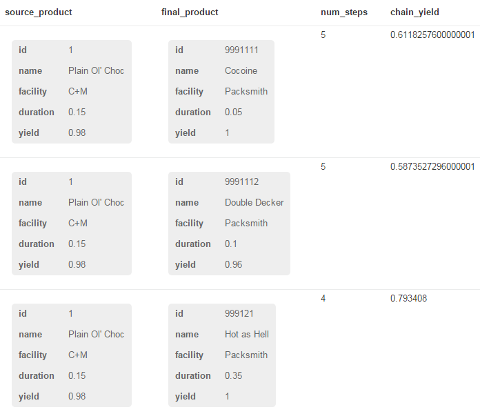
This data is reasonable because I doctored the product identifiers to begin with 999 for the products that are shipped to customers and when a product becomes another (though the MOVES_TO relationship) a unique positive integer is added to the original product’s code. So, id 999124 means that it is a final product, and it the fourth product that descends from 12, which descends from 1. You can of course compute the yield across a hierarchy in a relational database such as Oracle too, as I explained before. There is no real technical advantage, except that a graph database stores the data in a format that is close to what it actually represents, which may be beneficial to the performance. Where a graph database such as Neo4j really shines is when you want to see the how all the branches of a directed acyclic graph are connected, which is a tough nut to crack in pure SQL. Here’s how to get every product that’s somehow connected to Cheapo Choc:

MATCH
  p=(s)-[:MOVES_TO*]-(t)
WHERE
  s:Product
  AND s.name = 'Cheapo Choc'
RETURN
  nodes(p) AS path

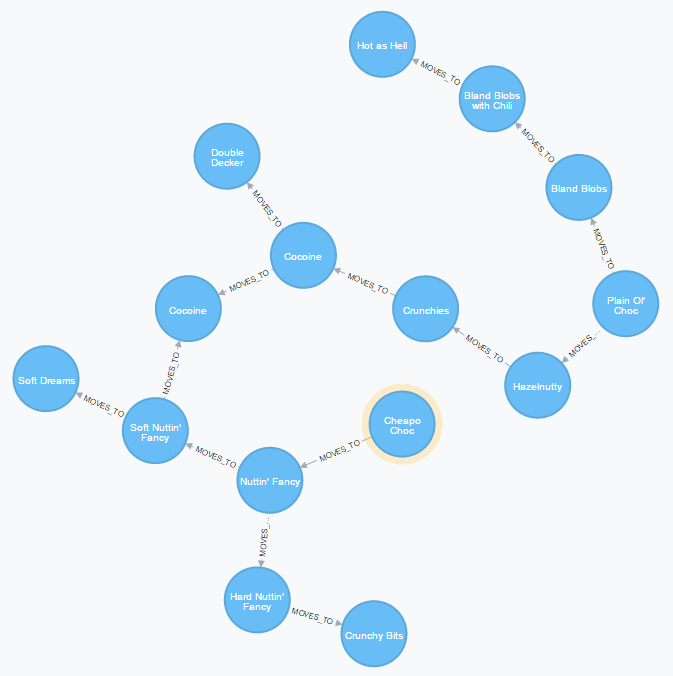
Please check the relationship again: it has no arrow, so it asks for any MOVES_TO relationship without regard for the direction between s and t. A relational database would have tremendous difficulty obtaining such a graph in tabular form because CONNECT BY and recursive common table expressions look only in one direction: you pick the root of a tree and it simply goes up the trunk to the leaves. In the case of CONNECT BY it’s the PRIOR keyword that kills bi-directional search. Sure, you could check at each level that goes away from the root whether there are any incoming branches but that is horribly inefficient in complex networks. It is unlike the nested hierarchies solution that I compared previously, which — Surprise! — turned out to be the worst in terms of performance.

Cycle Time Over a Product Chain

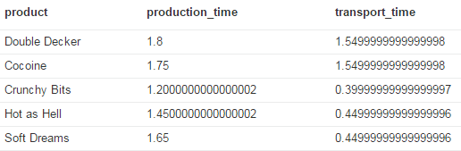
Another interesting query to build for a value stream or supply chain is the total cycle time for a particular product or simply all products:

MATCH
  p=(s:Product)-[:MOVES_TO*]->(t:Product)
WHERE
  NOT ()-[:MOVES_TO]->(s)
  AND NOT (t)-[:MOVES_TO]->()
RETURN
  t.name                                                        AS product
, MAX(reduce(pt = 0, n IN nodes(p) | pt + n.duration))          AS production_time
, MAX(reduce(tt = 0, r IN relationships(p) | tt + r.transport)) AS transport_time

In the query I have used a slightly different notation with regard to specifying the node type in the MATCH instead of the WHERE clause, merely to show off the flexibility of Cypher. The MAX aggregation function is required to make sure we take the longest production and transport time for each final product in case a product is made by combining different intermediate products. For instance, Cocoine is made by combining Cocoine from the Nougateria facility and Soft Nuttin’ Fancy. The former takes 1.70 days of production and 1.55 days of transport, whereas the latter requires 1.40 and 0.65 days, respectively. Add to that the production time of 0.05 days in the Packsmith facility, and you arrive at the numbers shown below.

Tracking Down Supplier Issues

Suppose one customer, say, ‘Noshes & Nibbles’ complains about the Hot as Hell chocolates. You suspect a supplier issue, so you want to see what suppliers are involved in the production of Hot as Hell:

MATCH
  path=(s:Supplier)-[*]->(p:Product { name: 'Hot as Hell'} )<-[:REQUIRES]-(c:Customer)
RETURN
  path

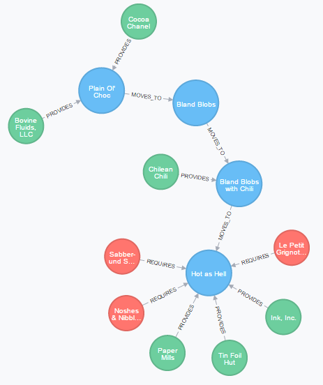
Since we want to see all paths that lead to Hot as Hell, we don’t care about (i.e. specify) the relationship type. Moreover, we want to see all potentially affected customers, hence the final relation in the MATCH clause. In case of poison in one of the raw materials, we need to inform all customers immediately, so it makes sense to list all who ordered Hot as Hell chocolate.

In itself the query gives a nice visual representation of the situation, but what if we wanted to see a list of suppliers and a list of affected customers. Some suppliers could possibly be used in different sections of the supply chain, so we’d want to list the unique nodes, both suppliers and customers. For complex supply chains, the graph may not be as useful. As an easy-peasy exercise, just try Cocoine instead of Hot as Hell.

Well, this should do it:

MATCH
  path=(s:Supplier)-[*]->(p:Product { name: 'Hot as Hell'} )<-[:REQUIRES]-(c:Customer)
RETURN
  p                        AS product
, collect(DISTINCT s.name) AS supplier_list
, collect(DISTINCT c.name) AS customer_list

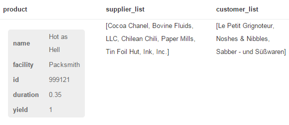
The collect function is an aggregation function that creates a list of whatever is provided as its argument. Unfortunately, you cannot sort the results as in Oracle’s LISTAGG.

Anyway, that’s all folks! I hope you can do something useful when modelling supply chains or value streams in Neo4j. Of course you can use similar techniques to model individual lots for tracability, which is not much more difficult that what I’ve described in this post.