Numerical Algorithms: Variational Integrators
When I was rummaging through my digital attic I found code that I had worked on a few years ago. It is not related to data or database technologies but it is in itself interesting, so that I thought I’d better share it.
To calculate integrals in mathematics or solve differential equations in physics or chemistry you often need a computer’s help. Only in very rare cases can you express the integral symbolically. In most instances you have to be satisfied with a numerical solution, which for many problems is perfectly fine.
The essence of numerical integrators is that they discretize the ordinary differential equations they try to solve, thereby making it easy for a computer to do the sums. There are of course many types of algorithms to solve differential equations, the most common being the integrators of the Runge-Kutta family. Classical integration algorithms also include multi-step methods, such as Adams-Bashforth-Moulton’s. What these methods have in common is that, as they progress with the computation, they accumulate discretization errors. Ad infinitum. Stated differently, the longer the time horizon, the bigger the error.
For some applications, for example astronomical or cosmological simulations and also spacecraft missions, that is a huge problem. As the mistake you make in the orbits of celestial bodies or satellites increases, confidence in the solution decreases.
Fortunately, there are certain geometric numerical integrators (GNIs) that have been shown to have many desirable properties, the primary being that the errors they make are bounded. Consequently, you know that your solutions are off by no more than a certain number that you can either determine mathematically or by estimating it based on actual data.
The reason these algorithms have bounded errors is that they respect fundamental mathematical structures, in particular the differential geometric structures that underpin the dynamics. In case you have no idea what I am talking about, think of classical integrators as general-purpose algorithms that solve many problems, some obviously better than others, whereas geometric numerical integrators are designed to solve a specific subset of problems with greater accuracy than their classical counterparts. 1
A few low-order GNIs are well-known and have been studied extensively. However, in simulations you can rarely do something useful with these low-order algorithms. To create higher-order geometric numerical integrators, you have a few options:
- Take a general-purpose algorithm, modify it, and prove that it conserves the differential geometric properties;
- Concatenate several lower-order GNIs such that error terms cancel out one another;
- Look at variational integrators.
Variational integrators do what GNIs do, but they derive from a so-called variational principle, which is a recurring theme in theoretical physics. You may have heard of the principle of least action or more aptly the principle of stationary action, which is what it is all about. The salient details are highlighted in a poster from the International Symposium on Symbolic and Algebraic Computation. It is geared towards for the more maths-savvy among you:
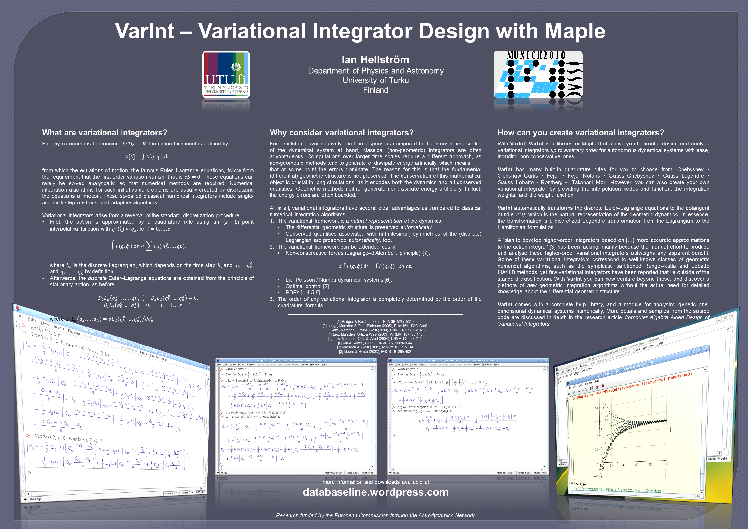
The Wordpress URL printed on the poster is obviously no longer valid.
The poster also shows screenshots from Maple, a computer algebra system, that I used to generate higher-order variational integrators. You see, the beauty of the variational formalism is that higher-order algorithms do not arise as magic cancellations of error terms in series expansions. Instead they come from using better approximations to calculate the discretized action. Nevertheless, researchers had mainly focused on either the mathematical aspects of variational integrators or practical implementations. Even though the formalism lends itself perfectly to the generation of higher-order algorithms, very few people actually derived higher-order integrators from the variational principle. I know of one such example of a fourth-order integrator in the astrophysics community, and that’s it. Most mathematicians have been completely satisfied with knowing that it is in principle possible to obtain higher-order algorithms but very few have done so. Enter VarInt.
With VarInt you specify the quadrature rule or interpolation function and the number of points you want to use, and it computes the numerical algorithm for you. What it does in the background is compute the discrete Euler-Lagrange equations. Alternatively, you can provide VarInt with the weights and locations for your own quadrature rule in case you want to use a scheme that is not built in. The details of the Maple code can be found in an abstract that accompanied the poster shown before, a conference paper, or my magnum opus called Numerics of Spacecraft Dynamics, which deals with the subject in a great more detail.
The following quadrature rules are supported up to arbitrary order, although I cannot imagine anyone going beyond tenth, for virtually all higher-order algorithms are implicit:
- Newton-Cotes
- Romberg
- Chebyshev
- Gauss-Legendre
- Gauss-Lobatto
- Fejér I-IV
- Clenshaw-Curtis
- Takahasi-Mori
VarInt also comes with a module (IntegrateSystem) that can be used to numerically integrate a dynamical system of your choice with a variational integrator that VarInt spits out, which is convenient because you can compare its performance without having to code a damn thing yourself.
All within Maple.
If you wish to run the Maple code as a fully integrated package, then please download it from the Maplesoft Application Centre and follow the instructions.
Additionally, I invite you to check out the code on GitHub.
The VarInt library on the repository is Release 6, which does not include extended support for exponential integrators, built-in Birkhoff interpolation algorithms, and an automatic translation (and code optimization feature) of the algorithms into #include-able C++ code, which is what I had been working on before both the funding and my patience ran out.
I may one day create a seventh release with these features but I shall not hold my breath.
-
For those who know about automatic or algorithmic differentiation (AD), integrators based on discretizations may seem like a crude method from the Stone Age to solve differential equations. However, automatic differentiation requires considerably more memory and horsepower, which for large-scale simulations and on-board attitude and orbit control software (AOCS) is not always possible. Moreover, support for special functions in commercial AD libraries is often limited. ↩