What Makes A New York Times Article Popular? (Part 2/2)
In the previous post I talked about the details of the data set for the Kaggle challenge to build a model that predicts which New York Times blog articles become popular. In this post I shall discuss how I went about to discover and add features, and build a predictive model that landed me in the top 15% of all entries.
Feature Engineering
Feature engineering is a fancy term for the ‘magic’ that is necessary to improve machine learning algorithms. It is the secret sauce that makes some analytical models stand out from the pack. From reading the forums afterwards I often had a why-didn’t-I-think-of-that moment when seeing a feature I did not have. Successful engineered features are often ‘obvious’ ex post facto, but before you have the aha moment they are typically hard to come up with.
So, how do you go about finding new features?
That’s a tough one. Sure, domain knowledge helps but hunches are helpful too. I know, hunches don’t appear out of thin air; they usually require a good deal of experience, which is something I cannot rely on too much, so I have to do it the hard way: trial and error.
Domain Knowledge
Since we are talking about blog posts on the New York Times, we can already use information about articles on the internet. For instance, we can introduce a variable that tells us whether the title would be truncated in search results, assuming that people land on the New York Times by googling:
News$SEO = as.factor(ifelse(News$HeadlineCharCount<=48, 1, 0))
The reason I pick 48 rather than 65 is that 48 allows the suffix ‘ - NYTimes.com’ to be added, which may or may not influence people’s decision to click and eventually comment on a particular article when they see it in the list of search results. It probably does influence people’s behaviour, as the mean popularity is in favour of the 48-character limit: 0.173 against 0.207.
Moreover, in the first post I mentioned a few blog-specific clues in the headline: questions, how-tos, negative phrases, and the like. So, let’s add those features too:
News$Question    = as.factor(ifelse(grepl("?", News$Headline), 1, 0))
News$Exclamation = as.factor(ifelse(grepl("!", News$Headline), 1, 0))
News$HowTo       = as.factor(ifelse(grepl("^how to", News$Headline, ignore.case=TRUE), 1, 0))
News$Negative    = as.factor(ifelse(grepl("<(never|do not|dont|don't|stop|quit|worst)>",
                                      News$Headline, ignore.case=TRUE), 1, 0))
News$SpecialWord = as.factor(ifelse(grepl("<(strange|incredible|epic|simple|ultimate|great|sex)>",
                                      News$Headline, ignore.case=TRUE), 1, 0))
Note that I have included an exclamation mark as a marker too, as there are 25 articles in the training set with an exclamation mark in the headline, of which 8 are popular. Perhaps, the exclamation mark is also successful at grabbing people’s attention.
What is more, the question mark may appear anywhere in the headline.
I could have restricted myself to questions marks at the end of the headline but the difference in popularity is not spectacular, so that I’d rather go for the anywhere-? rather than the end-? only.
The analysis of the difference is easy with the analyseTerms(...) function from the initial post.
The \\ ensure that whatever is written in-between is a whole word an not part of a word.
No Comment & Recurring Topics
There is still more, we can simply look at the current articles on the New York Times and see whether some types of articles have comment sections enabled. Remember, popular in the context of this competition means 25 or more comments. Some articles never receive comment sections for whatever reason, so we can look for those.
One way to do this — and the one I used — is to use the UnpopularNewsTrain data frame, sort by the headline, and then verify whether a certain class of articles never has a comment section.
sort(UnpopularNewsTrain$Headline)
That way, you’ll quickly see recurrent items that will never appear popular in this context, which we can easily capture with an additional feature:
News$NoComment = as.factor(ifelse(grepl(
  paste0("6 q's about the news|daily|fashion week|first draft|in performance|",
         "international arts events happening in the week ahead|",
         "inside the times|lunchtime laughs|pictures of the day|playlist|",
         "podcast|q. and a.|reading the times|test yourself|",
         "throwback thursday|today in|the upshot|tune in to the times|",
         "tune into the times|under cover|verbatim|walkabout|weekend reading|",
         "weekly news quiz|weekly wrap|what we're (reading|watching)|",
         "what's going on in this picture|word of the day"),
  News$Headline, ignore.case=TRUE), 1, 0))
Similarly, we can take a play peek-a-boo with PopularNewsTrain to identify recurrent items that are receive many comments:
News$Recurrent = as.factor(ifelse(grepl(
  "^(ask well|facts & figures|think like a doctor|readers respond|no comment necessary)",
  News$Headline, ignore.case=TRUE), 1, 0))
Although analyseTerms(...) tells us that only 12 such articles exist in the test set, 65.4% of the posts in the training set are popular.
Sticking the grepl string in analyseTerms(...) we can easily see that the training set has 829 such articles and the test set 254.
This means that we can expect roughly 13.6% of all articles in the test set to be classified correctly based on this single feature.
Politics & Controversies
Since we are dealing with newspaper blog articles, we can typically assume something about the readership: they are likely interested in (national) politics and there are likely some controversies. Luckily for us, the USA has several decade-old controversies that we can easily capture in a feature: gun control, abortion, racial issues.
News$Controversial = as.factor(ifelse(grepl(
  paste0("<(gun control|abortion|birth control|",
         "consent|rape|african-american|latino|racis(m|t))>"),
  News$Headline, ignore.case=TRUE), 1, 0))
The number of articles in our test data is a meagre 9. Still, we can use the feature and see whether it has a positive impact on the accuracy of our model. A topic that was current during the data was the police shooting of Michael Brown in Ferguson, Missouri. We can either choose to capture this topic in a separate variable or let the bag of words sort it out. For the time being, we shall leave it as is because it is not one of the age-old controversies in the US. Ebola is another news item that was on everyone’s radar in 2014.
Some political topics are often debated.
To identify the ones that are clearly above or below the mean, we have to figure out the mean.
We can take the politics grepl from the previous post and see that when searching both the headline and abstract for these terms, we have a probability of about 14.6% for any random post to be popular.
From analysing the various terms, I have come up with the following features:
News$Obama       = as.factor(ifelse(grepl("obama|president", News$Headline, ignore.case=TRUE), 1, 0))
News$Republican  = as.factor(ifelse(grepl("republican", News$Headline, ignore.case=TRUE), 1, 0))
News$Congress    = as.factor(ifelse(grepl("<(senate|congress)>", News$Headline, ignore.case=TRUE), 1, 0))
News$Election    = as.factor(ifelse(grepl("<(election|campaign|poll(s|))>", News$Headline, ignore.case=TRUE), 1, 0))
The danger with this approach is that when a particular topic or politician loses its edge or suddenly bursts outs into a heated debate due to a contoversy, we have no way of capturing that. All this accomplishes is grouping topically similar articles together. We could of course rely on a Latent Dirichlet Allocation (LDA) based on a term-document matrix, but more on that later.
Holidays
When people are not required to show up at work, they may be more inclined to read and comment on blog posts. So, perhaps there is a correlation between the holidays and the popularity of articles. Since we know the holidays and the time frame of the data set, we can easily do the following:
Holidays = c(as.POSIXlt("2014-09-01 00:00", format="%Y-%m-%d %H:%M"),
             as.POSIXlt("2014-10-13 00:00", format="%Y-%m-%d %H:%M"),
             as.POSIXlt("2014-10-31 00:00", format="%Y-%m-%d %H:%M"),
             as.POSIXlt("2014-11-11 00:00", format="%Y-%m-%d %H:%M"),
             as.POSIXlt("2014-11-27 00:00", format="%Y-%m-%d %H:%M"),
             as.POSIXlt("2014-12-24 00:00", format="%Y-%m-%d %H:%M"),
             as.POSIXlt("2014-12-25 00:00", format="%Y-%m-%d %H:%M"),
             as.POSIXlt("2014-12-31 00:00", format="%Y-%m-%d %H:%M"))

News$Holiday = as.factor(ifelse(News$PubDate$yday %in% Holidays$yday, 1, 0))
Interestingly, from looking at table(News$Popular, News$Holiday) we do not seem to get the impression that there is a huge difference in the popularity based on whether the publication date is a national holiday.
Still, we can keep the feature and remove it if it turns out to be unhelpful.
This observation may in itself be not too surprising. After all, on the holiday itself many people visit friends and family, so that reading and especially commenting is unlikely. What is likely is that people comment more on the evening before the public holiday, because they can stay up late.
Remember that from 7PM onwards, the mean popularity of articles increases almost linearly. Is this time of day at all logical? Well, most people leave work around 5PM, they commute back home, perhaps pick up the kids, exercise, and have dinner, which means that 7PM is a fairly sensible time for all that to have happened in-between. At 7PM some people may catch up on articles and post comments where appropriate. In the car or on the New York subway you may not have enough space to participate in a lengthy discourse on the economic outlook of Southeast Asia. As more and more people on the East Coast join in on the conversation, the sound of the factory whistle is heard in more parts of the United States. Hence, we can explain, or at least argue, why the mean popularity increases up to around 10PM, which happens to be 7PM on the West Coast.
Perhaps, we can introduce a feature that checks whether the article was posted in the 5 hours leading up to a public holiday. That can be accomplished as follows:
News$BeforeHoliday = as.factor(ifelse(News$PubDate$yday %in% (Holidays$yday-1) &
                                          News$PubDate$hour>=17, 1, 0))
The disadvantage is that the number of articles for which the variable is non-zero is fairly small. Let’s not worry about that now though.
Going Through Headlines and Abstracts
Since I have reached the limits of my ‘domain knowledge’, all that remains is going through the data. Manually.
News$Current = as.factor(ifelse(grepl(
  "ebola|ferguson|michael brown|cuba|embargo|castro|havana",
  News$Text, ignore.case=TRUE), 1, 0))

News$Cuba = as.factor(ifelse(grepl("cuba|embargo|castro|havana",
                                     News$Text, ignore.case=TRUE), 1, 0))

News$Recap = as.factor(ifelse(grepl("recap",
                                       News$Headline, ignore.case=TRUE), 1, 0))

News$UN = as.factor(ifelse(grepl("u.n.|united nations|ban ki-moon|climate",
                                      News$Text, ignore.case=TRUE), 1, 0))

News$Health = as.factor(ifelse(grepl(
  paste0("mental health|depress(a|e|i)|anxiety|schizo|",
         "personality|psych(i|o)|therap(i|y)|brain|autis(m|t)|",
         "carb|diet|cardio|obes|cancer|homeless"),
  News$Headline), 1, 0))

News$Family = as.factor(ifelse(grepl(
  "education|school|kids|child|college|teenager|mother|father|parent|famil(y|ies)",
  News$Headline, ignore.case=TRUE), 1, 0))

News$Tech = as.factor(ifelse(grepl(
  paste0("twitter|facebook|google|apple|microsoft|amazon|",
         "uber|phone|ipad|tablet|kindle|smartwatch|",
         "apple watch|match.com|okcupid|social (network|media)|",
         "tweet|mobile| app "),
  News$Headline, ignore.case=TRUE), 1, 0))

News$Security = as.factor(ifelse(grepl("cybersecurity|breach|hack|password",
                                         News$Headline, ignore.case=TRUE), 1, 0))

News$Biz = as.factor(ifelse(grepl(
  paste0("merger|acqui(s|r)|takeover|bid|i.p.o.|billion|",
         "bank|invest|wall st|financ|fund|share(s|holder)|market|",
         "stock|cash|money|capital|settlement|econo"),
  News$Headline, ignore.case=TRUE), 1, 0))

News$War = as.factor(ifelse(grepl(
  paste0("israel|palestin|netanyahu|gaza|hamas|iran|",
         "tehran|assad|syria|leban(o|e)|afghan|iraq|",
         "pakistan|kabul|falluja|baghdad|islamabad|",
         "sharif|isis|islamic state"),
  News$Text, ignore.case=TRUE), 1, 0))


News$Holidays = as.factor(ifelse(grepl("thanksgiving|hanukkah|christmas|santa",
                                         News$Text, ignore.case=TRUE), 1, 0))

News$Boring = as.factor(ifelse(grepl(
  paste0("friday night music|variety|[[:digit:]]{4}|photo|today|",
         "from the week in style|oscar|academy|golden globe|diary|",
         "hollywood|red carpet|stars|movie|film|celeb|sneak peek|",
         "by the book|video|music|album|spotify|itunes|taylor swift|",
         "veteran|palin|kerry|mccain|rubio|rand paul|yellen|partisan|",
         "capitol|bush|clinton|senator|congressman|governor|chin(a|e)|",
         "taiwan|tibet|beijing|hongkong|russia|putin"),
  News$Text, ignore.case=TRUE), 1, 0))
Disclaimer: no judgements are intended based on the naming of the variables.
Random Forest
I tried several of the models discussed in the course: logistic regression, CART, and random forests. The random forests performed best consistently, so I shall not linger on the others.
After we have cleaned up our data frames (i.e. removed stuff we don’t need), we can simply run the following command:
rfModel = randomForest(Popular ~ ., data=NewsTrain, nodesize=5, ntree=1000, importance=TRUE)
The model can be tuned and cross-validated with the train function of the caret package like so:
trainPartition = createDataPartition(y=NewsTrain$Popular, p=0.5, list=FALSE)
tuneTrain      = NewsTrain[trainPartition, ]
rfModel.tuned  = train(Popular ~ .,
                   data=tuneTrain,
                   method="rf",
                   trControl=trainControl(method="cv", number=5))
What I found was an accuracy of 0.916 for mtry equal to 47.
The importance of every variable can now be plotted as follows:
imp = melt(importance(rfModel, type=1))
imp$sign = ifelse(imp$value>=0, "positive", "negative")

ggplot(imp, aes(x=reorder(Var1, value, max), y=value, group=Var2, fill=sign)) +
  geom_bar(stat="identity") +
  coord_flip() +
  ggtitle("Relative Importance of Predictors") +
  theme(axis.title.y = element_blank()) +
  ylab("Mean Decrease Accuracy") +
  theme(legend.position = "none")
A simple call to varImpPlot(rfModel, type=1) would have worked too, but the resulting graph is not as pretty.
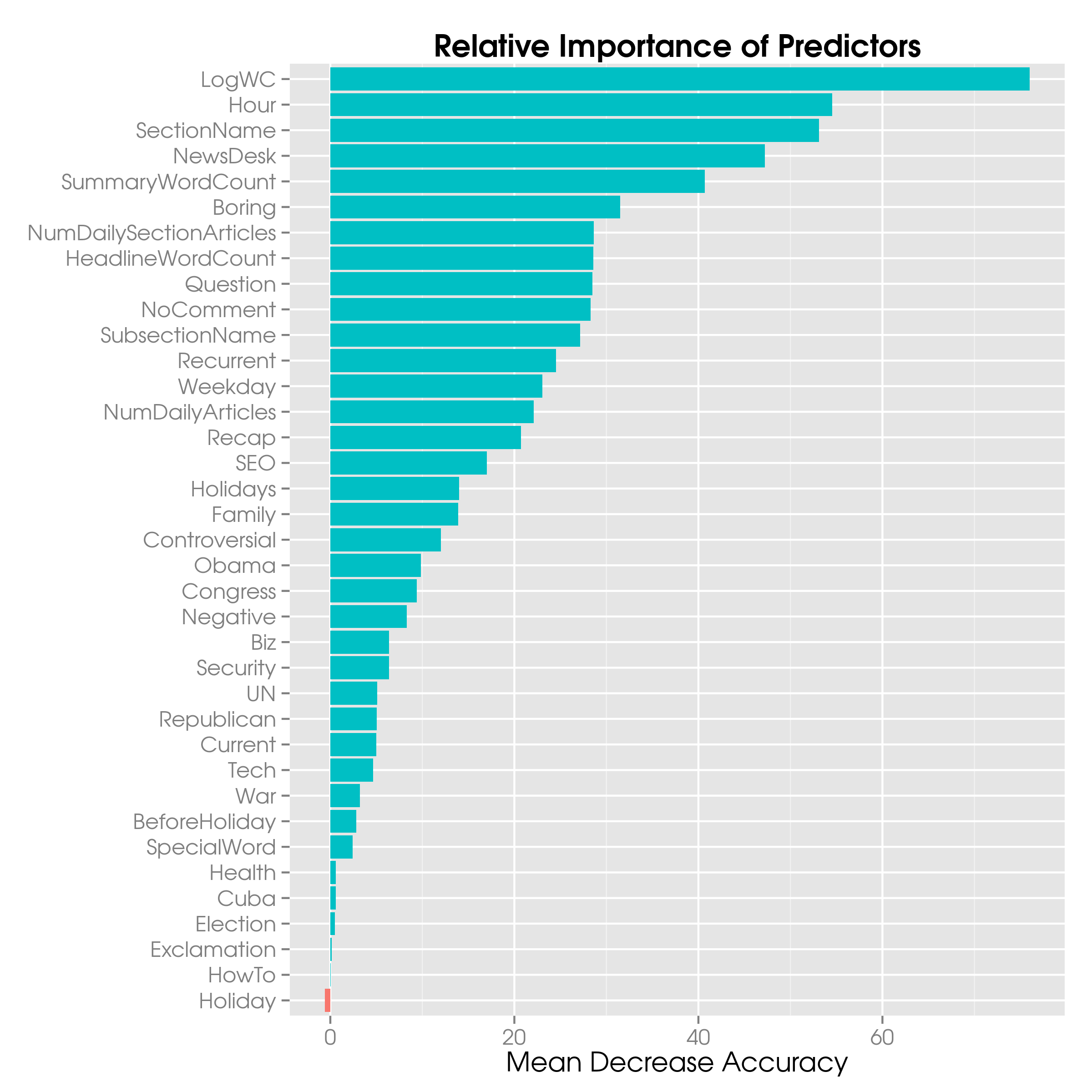
What this plot shows is that most variables have a positive contribution, whereas some have a negative.
In particular, Health does not seem to be a healthy predictor for the random forest.
Please observe that BeforeHoliday, though very few posts have a non-zero value of it, is higher up the list than Holiday.
The negative contribution of Holiday is most likely due to the correlation between both variables.
What we can do is drop Health as well as Holiday and see what that does for the importance of the variables.
But before we do that, let’s calculate the accuracy and AUC on the training set:
calcAUC = function(model, truth)
{
  suppressPackageStartupMessages(require(ROCR))

  model.predTrain = predict(model, type="prob")
  model.accuTrain = tr(table(truth, model.predTrain[, 2]>0.5))/nrow(model.predTrain)
  model.aucTrain  = as.numeric(performance(prediction(model.predTrain[, 2], truth), "auc")@y.values)

  return(c(model.accuTrain, model.aucTrain))
}

calcAUC(rfModel, NewsTrain$Popular)
We find that the training accuracy and AUC are 0.917 and 0.946, respectively.
When we drop Health and Holiday we see that the accuracy and AUC become 0.918 and 0.945.
What is more interesting is that now the contribution of Cuba is positive. HowTo is barely positive, so we may be able to drop it without losing much, and indeed, if we do, the accuracy and AUC are pretty stable; Cuba’s contribution becomes negative again though.
After getting rid of Cuba (and Election whose contribution turns out to be negative) we obtain 0.919 and 0.947 for the accuracy and area under curve, respectively.
These tweaks would have given a test AUC of 0.89317, which would have been worthy of the 771st place on the leader board.
An (overfitted) logistic model with exactly the same variables would have scored 0.89194 and landed in 865th position.
Text Mining
So far, we have only added features by manual inspection of the text fields supplied.
We can of course use the tm package to do the hard work for us.
We can leave the features that have nothing to do with looking through the text fields, so that we do not run into interdependencies issues.
Since mainly headlines grab someone’s attention and the abstract is a short summary of what’s in the full article, it seems to make sense to split the corpora based on the headline and abstract, or rather the summary. We can do that as follows:
dropWords = c(stopwords("SMART"))

CorpusHeadline = Corpus(VectorSource(News$Headline))
CorpusHeadline = tm_map(CorpusHeadline, tolower)
CorpusHeadline = tm_map(CorpusHeadline, PlainTextDocument)
CorpusHeadline = tm_map(CorpusHeadline, removePunctuation)
CorpusHeadline = tm_map(CorpusHeadline, removeWords, dropWords)
CorpusHeadline = tm_map(CorpusHeadline, stemDocument, language="english")
dtmHeadline = DocumentTermMatrix(CorpusHeadline)
sparseHeadline = removeSparseTerms(dtmHeadline, 0.995)
sparseHeadline = as.data.frame(as.matrix(sparseHeadline))
colnames(sparseHeadline) = make.names(paste0("H",colnames(sparseHeadline)))

CorpusSummary = Corpus(VectorSource(News$Summary))
CorpusSummary = tm_map(CorpusSummary, tolower)
CorpusSummary = tm_map(CorpusSummary, PlainTextDocument)
CorpusSummary = tm_map(CorpusSummary, removePunctuation)
CorpusSummary = tm_map(CorpusSummary, removeWords, dropWords)
CorpusSummary = tm_map(CorpusSummary, stemDocument, language="english")
dtmSummary = DocumentTermMatrix(CorpusSummary)
sparseSummary = removeSparseTerms(dtmSummary, 0.99)
sparseSummary = as.data.frame(as.matrix(sparseSummary))
colnames(sparseSummary) = make.names(paste0("S",colnames(sparseSummary)))

NYTWords                         = cbind(sparseHeadline, sparseSummary)
NYTWords$Popular                 = News$Popular
NYTWords$NewsDesk                = News$NewsDesk
NYTWords$SectionName             = News$SectionName
NYTWords$SubsectionName          = News$SubsectionName
NYTWords$LogWC                   = News$LogWC
NYTWords$Weekday                 = News$Weekday
NYTWords$Hour                    = News$Hour
NYTWords$SEO                     = News$SEO
NYTWords$Question                = News$Question
NYTWords$Holiday                 = News$Holiday
NYTWords$BeforeHoliday           = News$BeforeHoliday
NYTWords$NumDailyArticles        = News$NumDailyArticles
NYTWords$NumDailySectionArticles = News$NumDailySectionArticles
NYTWords$NumHourlyArticles       = News$NumHourlyArticles

NYTWordsTrain = head(NYTWords, nrow(NewsTrain))
NYTWordsTest  = tail(NYTWords, nrow(NewsTest))
These command create the corpora based on the term frequency.
We can supply control=list(weighting=weightTfIdf) to the call to DocumentTermMatrix to create corpora based on the term frequency–inverse document frequency (tf-idf).
Terms that appear in most posts are probably not that revealing, so that the inverse document frequency can take care of these.
I have played around with this option but the results have not been too different from the standard approach.
Please notice the difference in the values for the sparsity.
Since headlines are read more often it makes sense to include a few more terms.
I have included News$Question and the like because the bag-of-words model cannot discover these features from the plain text.
Before we build our random forest, let’s take a few minutes to look at the most frequent terms and find associations. First, the term frequencies:
freqTerms = findFreqTerms(dtmHeadline, lowfreq=100)
termFreq  = colSums(as.matrix(dtmHeadline))
termFreq  = subset(termFreq, termFreq>=100)
df        = data.frame(term=names(termFreq), freq=termFreq)

ggplot(df, aes(x=reorder(term, freq, max), y=freq)) +
  geom_bar(stat="identity") +
  ggtitle("Most Common Terms in the Headline") +
  xlab("Terms") +
  ylab("Frequency") +
  coord_flip()
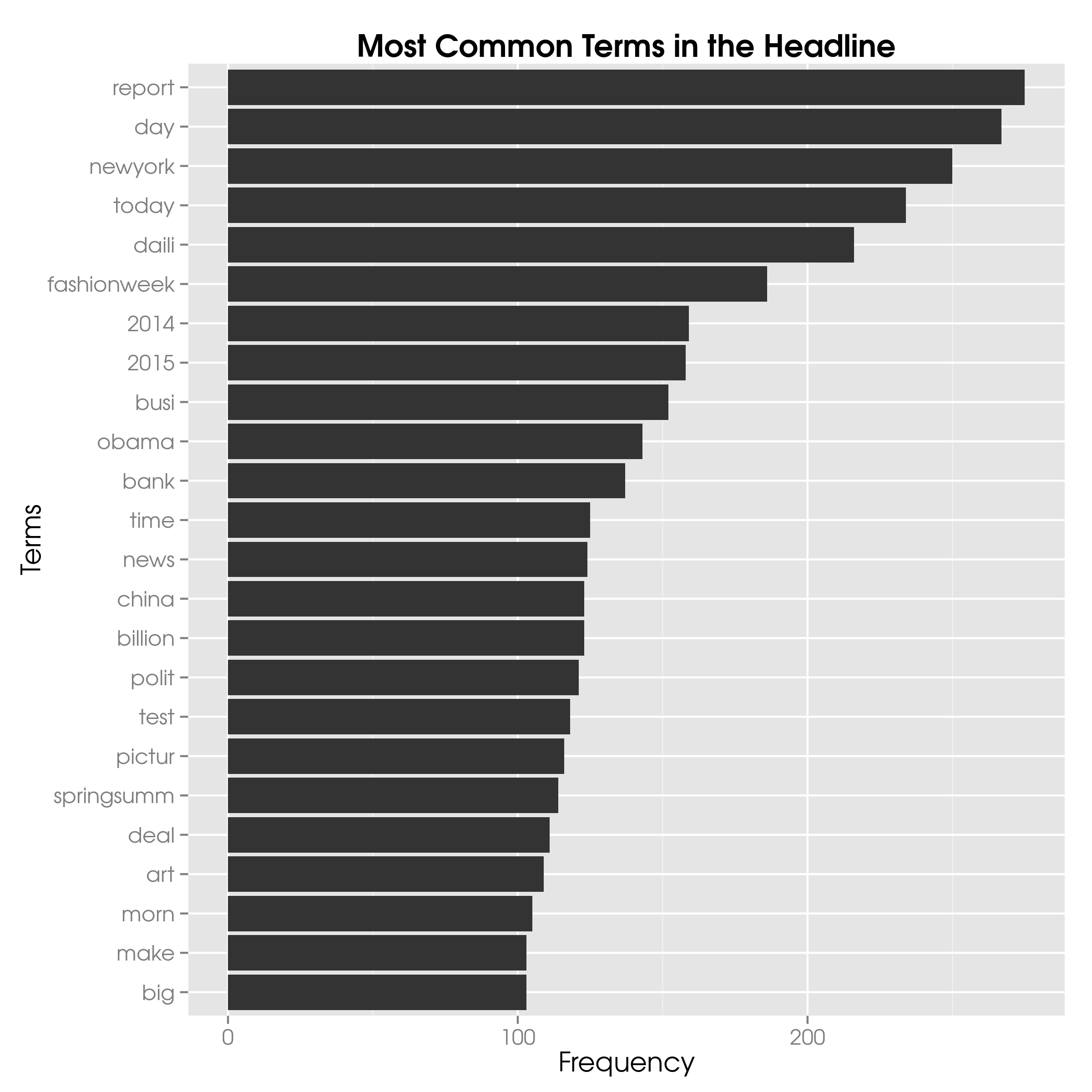
We see that the word ‘report’ is the most common in all headlines, appearing in 275 articles.
The term ‘day’ is also quite popular in headlines with 267 entries, although we could remove it by adding it to our dropWords vector.
It seems after all highly unlikely that the appearance of ‘day’ makes a difference in article popularity.
Nevertheless, analyseTerms("\\") returns a mean popularity of 0.03, so the term is indicative of unpopular news items, which means that including it as a feature does make sense.
Next, we can look at associated words.
For instance, findAssocs(dtmHeadline, "obama", 0.1) gives us words in the headline that are frequently associated with Barack Obama. ‘Michelle’ seems to be most commonly associated word, which happens to be his wife’s first name.
Moreover, we find ‘immigr’, which is the stem of immigration and immigrant(s).
Interestingly, third on the list is ‘paltrow’, which seems to indicate the actress Gwyneth Paltrow.
Another one we can look at is one of the NoComment titles.
The combination ‘Throwback Thursday’ pops up from time to time, so let’s look at findAssocs(dtmHeadline, "throwback", 0.2), which gives us ‘thursday’, rather unsurprisingly.
Why can’t we look at ‘Fashion Week’?
Because we already remove the space between the words with custom mgsub function; the combination is already in our aforementioned chart with the top entries in the headline.
Anyway, these checks are encouraging.
A random forest with the same settings as before yields an accuracy of 0.906 when doing a five-fold cross validation on the training set with a 50-50 split, a training set accuracy of 0.917 and an AUC of 0.935, slightly lower. The AUC on the test set is 0.90417, which would have been 197th best entry. So, all the hard work in defining features was somewhat wasted as a simple bag-of-words random-forest classifier fared much better.
A call to varImpPlot(...) tells us that, again, the number of words in the article is the most important factor.
The five best indicators from the bag of words are music (headline), fashion week (headline), music (summary), share (summary), and show (summary).
By the way, anyone who has been paying attention will notice that this model has a better AUC than my ‘best’ model. It’s true. I did have a bag-of-words model that I had submitted but it did not include some of the features I would create later on. Both these blog entries are more structured in the hope that they benefit my dear readers; I hope the absence of chaos is for the best. The difference a more structured approach could have made in the final ranking proves I am sometimes as think as two short planks. Anyway, this clearly shows that analysing the data and thinking about the model carefully is what separates good models from acceptable models. Experience and instinct are probably what separates great models from the good ones.
Ensembles
Although a random forest is already an ensemble learning method in the sense that it constructs many decision trees and picks the locally best one, we can still blend several models together, for instance a logistic model and a random forest. The rationale for doing so is that it allows for different models to reinforce their decisions, where they agree, or in cases of doubt, use a majority vote or mean to pull an observation across the threshold, or do the opposite.
Suppose the test-set predictions for the random forest with custom features and bag of words are called rfCustomModel.PredTest and rfBoWModel.PredTest respectively, and the test-set predictions for the logistic model logModel.PredTest, we can combine the three as follows:
ensemblePred = (rfCustomModel.PredTest[, 2] + rfBoWModel.PredTest[, 2] + logModel.PredTest)/3
Of course, we can add different weights or even use a majority vote rather than the mean prediction. The blended AUC on the test set is 0.90573, which would have been number 132. As you can see, the blending improved the model slightly. Since the logistic model suffers from overfitting, we may want to reduce its influence on the final result by adding weights in favour of the random forests. For instance, when we take a 2-3-1 weighting (and thus divide by 6), the final AUC is 0.90623, which is the 123rd score on the leader board. Again, a slight improvement.
Let’s pause and think about what we have achieved so far. First, 90% of the time our model can differentiate between a randomly selected popular (true positive) and unpopular (true negative) article. Second, by combining different models, that is, models with different features and completely different algorithms to make predictions, we can improve upon the original accuracies of our individual models. Quite impressive, don’t you agree?
N-Grams
What about n-grams or combinations of words that appear often rather than just single words? Well, we can include them in the bag of words. For instance, we can look at monograms, bigrams and trigrams as follows — observe that I am sneaking in the tf-idf weighting too:
NGTokenizer    = function(x) NGramTokenizer(x, Weka_control(min = 1, max = 3))
tdmHeadline    = TermDocumentMatrix(CorpusHeadline,
                                    control=list(weighting=weightTfIdf,
                                                 tokenize=NGTokenizer))
tdmSummary     = TermDocumentMatrix(CorpusSummary,
                                    control=list(weighting=weightTfIdf,
                                                 tokenize=NGTokenizer))
We can use the Text variable but from the previous work we already have CorpusHeadline and CorpusSummary, so there is no need to build a new CorpusText, although I have included the code anyway:
CorpusText = Corpus(VectorSource(News$Text))
CorpusText = tm_map(CorpusText, tolower)
CorpusText = tm_map(CorpusText, PlainTextDocument)
CorpusText = tm_map(CorpusText, removePunctuation)
CorpusText = tm_map(CorpusText, removeWords, dropWords)
CorpusText = tm_map(CorpusText, stemDocument, language="english")
tdmText    = TermDocumentMatrix(CorpusText,
                                 control=list(weighting=weightTfIdf,
                                              tokenize=NGTokenizer))
names(tdm) = make.names(names(tdmText))
sparseText = removeSparseTerms(tdm, 0.99)
freqTerms  = findFreqTerms(sparseText, lowfreq=30)
termFreq   = rowSums(as.matrix(sparseText))
termFreq   = subset(termFreq, termFreq>=30)
df         = data.frame(term = names(termFreq), freq = termFreq)

ggplot(df, aes(x=reorder(term, freq, max), y=freq)) +
  geom_bar(stat="identity") +
  ggtitle("Most Common N-Grams in News$Text") +
  xlab("Terms") +
  ylab("Count") +
  coord_flip()
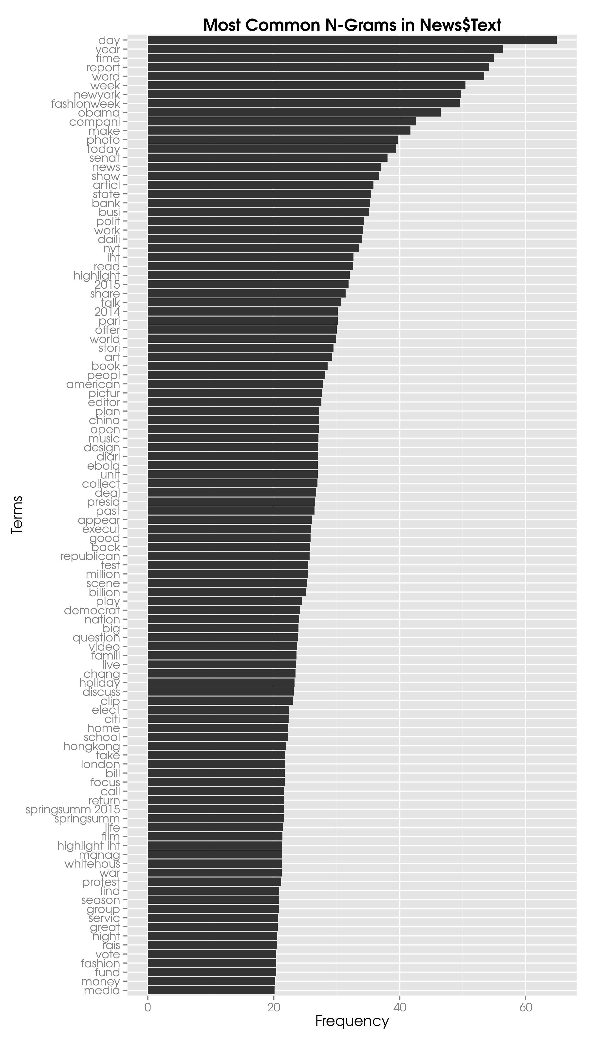
Since I have used the n-grams to identify a couple of phrases for the mgsub function, very few show up in the most frequent terms any longer.
There are, however, two stemmed combinations in headlines that appear together frequently: ‘springsumm 2015’ and ‘newyork today’ — ‘newyork’ and ‘fashionweek’ are near the top too.
The first bigram belongs to fashion week as the corresponding articles discuss the fashion trends for the next year’s spring-summer collections. ‘New York Today’ is likely a feature about the metropolitan area.
In the summary we find the most common combination to be ‘highlight iht’, which are highlights from the International Herald Tribute’s archives. Beyond that we observe ‘fashionweek photo diari’ or a photo diary of the various fashion week events.
In case you are interested to plot a dendrogram based on hierarchical clustering of the n-grams, the following code should help you on your way:
NYTNGrams.matrix     = as.matrix(sparseText)
NYTNGrams.distMatrix = dist(scale(NYTNGrams.matrix))
NYTNGrams.clusters   = hclust(NYTNGrams.distMatrix, method="ward")
plot(NYWords.clusters)
There is also the ggdendro package to plot dendrograms with ggplot2 rather than the standard plot command.
All you have to do is load it and run ggdendrogram(NYWords.clusters).
In case you want to stick with ggplot2 and not fuss with a wrapper, you can read about dendrograms here.
We can of course use k-means clustering too. An interesting way to use it is to generate clusters and see the words that make up these clusters. This is perhaps a poor man’s topic modelling approach, but it is worth the effort:
k   = 25
M   = t(sparseText)
KMC = kmeans(M, k)

for (i in 1:k) {
  cat(paste("cluster ", i, ": ", sep=","))
  s = sort(KMC$centers[i, ], decreasing=TRUE)
  cat(names(s)[1:15], sep=", ", "n")
 }
Here I have used 25 clusters. Well, I could look at the dendrograms and see where there is the most wiggle room, which is a simple explanation of what it typically comes down to. The dendrograms are, however, not exactly easy to analyse visually. The number 25 is large enough that several related topics are not lumped together, for instance elections and political items that have nothing to do with elections, and small enough that we can use the standard implementation of a random forest should we so desire.
What we see from running the loop are the first 15 words that define each cluster. Below is a snippet of the output:
cluster 1: bank, compani, deal, billion, market, ...
cluster 2: fund, bill, money, firm, invest, ...
cluster 3: court, rule, case, feder, decis, ...
cluster 4: talk, head, rule, morn, insid, ...
cluster 5: word, articl, clip, appear, daili, ...
.
.
.
cluster 24: school, student, children, test, start, ...
cluster 25: fashionweek, 2015 scene, springsumm 2015 scene, springsumm, springsumm 2015, ...
Cluster 1 is related to business, cluster 2 deals with investing and legislation, 3 belongs to jurisprudence, 4 is about general topics, and 5 has our word-of-the-day and similar recurrent pieces. Similarly, we see that the 24th cluster pertains to children and school and the final cluster is about fashion.
We can dump the clusters into our News data frame:
News$TopicCluster = as.factor(KMC$cluster)
And when we re-run the random forest, we find a slight improvement over the original model. The AUC on the full test set went from 0.89317 to 0.89799. For our 2-3-1 blended model, where we substitute the original random-forest model with the latest that includes the topic clusters, we obtain 0.90755, which is the 79th best submission on the leader board. If only…
Oh well, I passed the course with 91%, so I’m not too sad.
Topic Modelling
Wouldn’t it be nice to let an algorithm figure out the topics to which an article belongs based on the words in the headline and abstract (or summary)?
It sure would!
This could combat the issue with missing categories but also create clusters of articles based on topics.
We can of course manually create many features and do a k-means clustering.
The issue is that most features are binary factors, so the distance between News$Obama and News$Politics is the same as News$Food, although an article about Obama eating a cherry pie is unlikely to be written very often.
Not discussed in the edX course was topic modelling, a probabilistic technique for natural language processing (NLP). Latent Dirichlet Allocation (LDA) is a fairly recent invention that allows documents (i.e. articles) to be grouped based on words that appear together more often. The bag-of-words approach and LDA both assume the exchangeability of both words and documents. Phrased in perhaps somewhat more familiar terms: the order in which words or documents appear is completely irrelevant.
LDA can be used to extend our models but we can also use it to reduce the dimensionality: instead of having hundreds of words as individual features we can condense these words to a small set of topics. Fortunately, LDA is made very easy in R, as I discovered on these excellent slides by Yanchang Zhao.
dtmText      = DocumentTermMatrix(CorpusText)
ldaText      = LDA(dtmText, k=25) # 25 topics
topicTerms   = terms(ldaText, 5)  # first 5 terms for each topic
topicTerms   = apply(topicTerms, MARGIN=2, paste, collapse=", ")
topicsText   = topics(ldaText, 1)
News$Topic   = as.factor(topicsText)

topicsSeries = data.frame(date=as.Date(News$PubDate), topic=topicsText, terms=topicTerms[topicsText])

ggplot(topicsSeries, aes(x=date)) +
  geom_density(aes(y=..count.., fill=terms), position="stack") +
  ggtitle("Evolution of the Distribution of Topics") +
  xlab("Publication Date") +
  ylab("Frequency")

With the LDA topics instead of the k-means clusters the random-forest model scores a 0.89680 on the full test set, which is not an improvement. Inside our 2-3-1 blend the AUC becomes 0.90692. Again, not an improvement.
We can create a 4-model blend of the random forests with k-means clusters (3), the LDA topics (2) and the bag-of-words (4), and the overfitted logistic model (1); the weights are placed in parentheses. Its score is 0.90665 and lands on the 105th position. So, we see that the three-model blend from the previous section beats the random forest with the LDA-generated topics.
What is interesting to note is that in all models, WordCount, or rather the transformed LogWC, is the most important predictor of the popularity of a New York Times blog article, which leads us to the following conclusion:
TL;DR
If you happen to have a long piece, you’ll grab people’s attention.
In case you skipped all the way down to this section, you probably won’t understand the concluding double entendre, so you’ll have to go back and start over.
You’re welcome!